A Practical Guide to Elasticsearch Build Index for RAG

Building an Elasticsearch index is the first real step in creating a high-performance search system. It’s a process that involves defining core settings like shards and replicas, creating a data structure with mappings, and finally, ingesting your documents.

For Retrieval-Augmented Generation (RAG) systems, getting this right isn't just important—it's everything. A well-planned index is what makes the retrieval component both lightning-fast and dead-on accurate, ensuring the context fed to your LLM is of the highest quality.

The Architectural Blueprint for Your RAG Index

Building an Elasticsearch index for a RAG system is less about loading data and more about architecting a high-performance retrieval engine. The choices you make right at the beginning—from resource allocation to your data structure—will directly impact the speed, relevance, and scalability of your AI application down the line.

A poorly planned index inevitably leads to slow queries and irrelevant context being fed to the LLM, which completely undermines the "augmented" part of RAG. This foundational work ensures your data is not just stored, but actually optimized for the specific demands of AI-driven retrieval. You need to be thinking about:

• Scalability and Performance: How will the index handle growing data volumes and concurrent queries without increasing retrieval latency?
• Data Integrity and Availability: How will you protect against node failures to ensure the retrieval component of your RAG system is always online?
• Retrieval Relevance: How will the index be structured to retrieve the most semantically relevant and contextually rich information from your documents?

This simple workflow breaks down the high-level process for building an index that works.

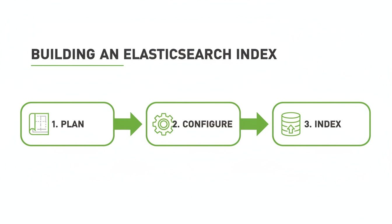
As you can see, successful indexing starts long before you load a single byte of data. It’s about being strategic, not just technical.

Planning Shards and Replicas for High Availability

One of the first and most critical decisions is configuring the number of shards and replicas. These settings directly control both retrieval performance and high availability.

By default, Elasticsearch creates an index with 1 primary shard and 1 replica. For production environments handling the large-scale data required for RAG systems, this is a recipe for poor performance and downtime.

A much better starting point is 3 primary shards and 2 replicas per index. This configuration ensures your cluster can distribute the retrieval load across multiple nodes while maintaining solid fault tolerance. Since replicas are never placed on the same node as their primary shard, a node failure means a replica can seamlessly take over without any data loss, keeping your RAG application's retrieval endpoint online.

To get a better sense of how crucial well-structured indexing is for information retrieval, it’s helpful to look at how modern Enterprise Document Management Solutions operate. Just as those systems need a solid foundation to manage critical business documents, your RAG system needs a robust index to retrieve precise information.

Think of shards as individual workers that divide and conquer the indexing and search load. More shards can boost retrieval performance by parallelizing queries, but only up to a point. Too many will just create unnecessary overhead. The trick is finding a balance that matches your data volume and query patterns.

Aligning Index Design with RAG Workflows

For any RAG application, your index absolutely must be designed to preserve the rich context generated during document processing. Your retrieval quality is only as good as the data you can access.

A generic index that flattens all data into a single text field throws away valuable metadata. This is a critical mistake. To enable advanced retrieval strategies like filtering by source or date, your index mapping needs to explicitly define fields for metadata. This traceability is what allows you to link a retrieved chunk back to its original source page, a crucial feature for validating context and building trust in RAG systems.

Core Index Settings for RAG Workflows

To get started, here's a quick-reference table that compares default Elasticsearch settings with my recommended configurations for a robust RAG system.

Setting	Default Value	Recommended for RAG	Why It Matters for Retrieval
number_of_shards	1	3 (or more, based on data size)	Distributes the workload for faster, parallelized query execution and better retrieval scalability. A good rule of thumb is 1 shard per 20-40GB of data.
number_of_replicas	1	2	Provides high availability for the retrieval endpoint and scales read operations, allowing more concurrent queries without performance degradation.
refresh_interval	1s	30s or -1 (during bulk ingest)	Reduces indexing overhead, freeing up cluster resources to serve retrieval requests faster. Frequent refreshes are costly and unnecessary until you need to query the data.

These settings aren't set in stone, but they provide a much stronger starting point for a production-ready RAG index than the out-of-the-box defaults. You'll want to adjust them based on your specific cluster size, data volume, and query load.

Designing Your Index Mappings for Precision Retrieval

Once you've planned out your index architecture—shards, replicas, and all that—it's time to get into the details of your mappings. This is where you hand Elasticsearch a precise blueprint for your data. You’re telling it exactly how to interpret and store every single field, which is the real difference between a retrieval system that understands your data and one that’s just guessing.

Relying on Elasticsearch's default dynamic mapping is a classic rookie mistake, especially for complex RAG workloads. Sure, it’s convenient for a quick test. You throw a document at it, and it tries to figure things out: "2024-01-01" becomes a date, "active" becomes a boolean, and pretty much everything else gets mapped as a text field with a .keyword sub-field. But this convenience comes at a steep price: inconsistent field types and terrible retrieval relevance down the road.

For RAG data, which is often a rich mix of text chunks, summaries, keywords, and structured metadata, letting Elasticsearch guess is a recipe for disaster. An explicit mapping isn't just a good idea; it's non-negotiable for building a reliable retrieval system.

The Problem with Letting Elasticsearch Guess

A few years back, Elasticsearch made a major shift: they disabled automatic index creation in production environments. This wasn't a random change. It was a direct response to a painful issue called "mapping explosion," where the dynamic mapping from the first few documents would lock in a terrible structure for all future data.

Imagine your first document has a version field with the value 1.0. Elasticsearch might map it as a float. Then, when a document with version: "1.0-beta" comes along, it gets rejected. This exact problem was rampant. In fact, production guidelines from platforms like Bonsai.io show that this auto-creation feature was responsible for around 70% of early user issues. By forcing developers to define their mappings upfront, they saw field type mismatches drop by 85% in large deployments. You can find more of these hard-won insights from the experts at Bonsai.io.

Defining Your Fields for RAG

In a RAG system, every field has a job to do in the retrieval process. Your mapping needs to reflect that by assigning the right data type. Let's break down the most important ones.

• text for Full-Text Search: This is for the content your users will search, like your chunk_text or summary. A text field gets analyzed—broken into words, lowercased, and stemmed—which is what allows a search for "running" to match documents containing "ran" or "runs." This forms the basis of keyword-based retrieval (BM25).
• keyword for Exact-Match Filtering: Use this for any metadata you’ll need for pre-retrieval filtering or post-retrieval aggregation. Think document_id, category_tags, or source_file. Unlike text, keyword fields are not analyzed. The entire value is treated as a single token, which is essential for the kind of precise filtering you can learn about in our guide to the Elasticsearch term query.
• dense_vector for Semantic Search: This is the heart of modern RAG. The dense_vector type is where you store the numerical embeddings generated from your text chunks. You must define the number of dimensions your model produces (e.g., 1536 for OpenAI's text-embedding-3-large) and the similarity metric to optimize retrieval.
• Numeric and Date Types: Don't forget the basics. Fields like page_number (integer), chunk_sequence (integer), or last_modified (date) need their correct types so you can run range queries and sort your retrieval results properly.

By explicitly defining each field type, you gain precise control over retrieval. You’re ensuring filters hit exact values, full-text search works on analyzed content, and semantic search has properly stored vectors to work with. This is foundational for a high-performing index.

A Practical Mapping Example for RAG Retrieval

Alright, let's turn theory into practice. Here’s a concrete JSON mapping for an index designed to hold chunked data, optimized for hybrid search in a RAG system.

{
  "mappings": {
    "properties": {
      "chunk_id": { "type": "keyword" },
      "document_id": { "type": "keyword" },
      "source_file": { "type": "keyword" },
      "chunk_text": {
        "type": "text",
        "analyzer": "english"
      },
      "text_embedding": {
        "type": "dense_vector",
        "dims": 1536,
        "index": true,
        "similarity": "cosine"
      },
      "page_number": { "type": "integer" },
      "tags": { "type": "keyword" },
      "created_at": { "type": "date" }
    }
  }
}

We’ve made some deliberate choices here. The chunk_text field uses the built-in english analyzer for better linguistic matching in keyword searches. For the text_embedding field, we've configured it for a 1536-dimension vector and set the similarity to cosine, a common and effective choice for text embeddings.

Critically, all the metadata fields (document_id, tags, etc.) are set as keyword. This guarantees they can be used for fast, exact-match filtering to narrow down the search space before running expensive vector queries, dramatically improving retrieval speed and relevance. A structure like this gives you a rock-solid foundation for both traditional keyword and modern semantic search.

Efficiently Ingesting Data with the Bulk API and Pipelines

Once your index mappings are dialed in, the next big job is actually getting your data into Elasticsearch. How do you load thousands—or even millions—of document chunks without bringing your cluster to its knees?

Indexing documents one by one might seem like an obvious starting point, but it’s painfully slow. For any serious RAG workflow, the network overhead will kill your performance. That approach just doesn't scale.

This is where the Bulk API becomes your best friend. It’s the go-to method for high-throughput data ingestion, letting you bundle thousands of operations (create, update, delete) into a single, efficient HTTP request. The difference is night and day.

Leveraging the Bulk API for RAG Workflows

The idea behind bulk indexing completely changed the game for building large-scale Elasticsearch indices. It slashes the API call overhead that makes individual inserts so sluggish. The Bulk API, which has been a mature feature since Elasticsearch 2.0 back in 2015, allows for batched operations that can boost throughput by an order of magnitude.

It's not uncommon to see ingestion rates hit 20,000-50,000 documents per second on pretty standard hardware.

In fact, indices populated with the Bulk API are often built up to 10x faster than those using a naive, one-by-one loop. When you’re working with data from a tool like ChunkForge, which exports neatly into formats like JSONL, the process becomes incredibly simple. You can explore how Elasticsearch's indexing capabilities have evolved in their own tutorials.

To get your data ready for a bulk request, you just need to structure it as a sequence of action/metadata pairs, each followed by the actual document source. And don't forget—the file has to end with a newline character.

Here’s what that looks like with a JSONL export:

{"index": {"_index": "rag-chunks-v1", "_id": "doc1-chunk1"}}
{"chunk_text": "This is the first chunk of text from document one.", "document_id": "doc1", "page_number": 1, "text_embedding": [0.1, 0.2, ...]}
{"index": {"_index": "rag-chunks-v1", "_id": "doc1-chunk2"}}
{"chunk_text": "This is the second chunk from the same document.", "document_id": "doc1", "page_number": 1, "text_embedding": [0.3, 0.4, ...]}

This format is lean and efficient. Each pair of lines is a self-contained instruction, making it easy to stream massive datasets directly into Elasticsearch without hogging memory.

Automating Data Enrichment with Ingest Pipelines

While the Bulk API handles raw speed, Ingest Pipelines bring the intelligence. An Ingest Pipeline is a series of processors that can modify or enrich your documents before they officially hit the index. This is a huge win for RAG systems because it lets you offload pre-processing tasks directly to Elasticsearch.

Think of it as a data assembly line. As each document flows through, different processors get to work.

• Grok Processor: Great for parsing and structuring text from logs or other unstructured messages.
• JSON Processor: Can extract and structure fields from a stringified JSON object.
• Inference Processor: This is a game-changer for RAG. You can point it at a trained machine learning model—like a sentence transformer—to automatically generate vector embeddings from your chunk_text field on the fly. This centralizes your embedding logic.
• Script Processor: Lets you apply custom logic with Painless scripting for anything more complex.

Using Ingest Pipelines really cleans up your data preparation code. Instead of running a separate script to generate embeddings and then sending the results over, you can do it all in one seamless step. This tidies up your architecture and makes your whole ingestion process more robust and easier to manage.

Building a Simple Ingest Pipeline

Let's say you want to automatically add a timestamp to every document chunk you index. You can define a pipeline with a simple set processor.

Here’s how you’d create it:

PUT _ingest/pipeline/add-ingestion-timestamp
{
  "description": "Adds a timestamp to each document",
  "processors": [
    {
      "set": {
        "field": "ingested_at",
        "value": "{{_ingest.timestamp}}"
      }
    }
  ]
}

Once that pipeline exists, just attach it to your bulk request by adding a pipeline parameter to the URL:

POST /_bulk?pipeline=add-ingestion-timestamp

And that's it. Every document sent in that request will automatically get an ingested_at field. While this is a basic example, it shows how pipelines can automate data enrichment without touching your client-side code. For a deeper look at building these kinds of automated systems, check out our guide on creating a complete RAG pipeline.

By combining the Bulk API with Ingest Pipelines, you create a fast, scalable, and intelligent ingestion process that’s perfect for any RAG system.

Validating and Monitoring Your Index Health

Building an Elasticsearch index isn't a one-and-done job. Think of your index as a living, breathing part of your infrastructure—one that directly dictates how well your RAG system performs. If it's unhealthy, you'll get slow, unreliable retrieval results. The only way to keep it a high-performing asset is through proactive validation and monitoring.

This process kicks off the second your bulk ingest finishes. You need to know, right away, that the data landed as expected. This isn't just about catching errors; it's about confirming the foundation your RAG application will depend on for every single query.

Initial Health Checks with Cat APIs

Your first line of defense is the _cat APIs. These are simple, text-based endpoints that give you a human-readable snapshot of your cluster's state. I always use them for a quick health check right after indexing a new dataset.

Start with GET /_cat/health?v. This command tells you the cluster status (green, yellow, or red), node count, and shard status. Green is the goal—it means all your primary and replica shards are allocated and happy. A yellow status means replicas are unassigned, which compromises the high availability of your retrieval system.

Next, zoom in on your new index. A couple of quick commands will give you the crucial details:

• GET /_cat/indices/your-index-name?v: This shows the index health, status (open/closed), document count, and total storage size. It’s the fastest way to confirm all your document chunks were actually ingested.
• GET /_cat/shards/your-index-name?v: Here, you get a detailed, shard-by-shard breakdown. You can see which node each shard is on, its state, and its size. This is a lifesaver for tracking down unassigned shards, which are the usual suspects behind a yellow or red cluster status.

If the document count from _cat/indices lines up with the number of chunks you intended to ingest, you’ve passed the first critical validation.

Deeper Monitoring for RAG Performance

After the initial sanity check, the focus shifts to ongoing performance. This is where you track the metrics that directly impact your RAG application's user experience—things like how fast new documents become searchable or how quickly queries come back.

You can use the built-in monitoring tools in Kibana or hook into external observability platforms like Prometheus and Grafana. The key is to watch the right metrics.

A healthy index isn't just one that's "up." It's one that consistently delivers fast, relevant results under load. For RAG, this means low query latency and efficient resource use are non-negotiable.

Here are the performance indicators I keep a close eye on for retrieval quality:

• Indexing Latency: How long does it take for a new document chunk to become searchable? If this is high, your RAG system is working with stale information.
• Query Latency: The time it takes for a retrieval request to complete. Spikes here directly slow down your LLM's response time and harm user experience.
• Resource Utilization (CPU & Memory): High CPU during retrieval can signal inefficient queries (like unfiltered vector searches). High JVM memory pressure can grind your nodes to a halt.
• Indexing Back-pressure: This happens when you’re trying to index data faster than the cluster can handle it, which leads to rejected requests and data gaps.

Setting Up Proactive Alerts

All that monitoring data is useless unless it drives action. The final piece of the puzzle is setting up alerts that flag potential issues before they turn into full-blown outages. You can configure these in Kibana to ping you on Slack, email, or other channels when a metric crosses a threshold you've defined.

At a minimum, I recommend setting up alerts for these common RAG performance killers:

• Cluster health drops to yellow or red.
• Query latency spikes above a certain threshold (e.g., 500ms).
• JVM memory pressure stays above 85% for more than a few minutes.
• Disk space on a node drops below 15%.

By monitoring proactively and setting up smart alerts, you move from a reactive, fire-fighting mode to a preventative one. This is how you ensure your Elasticsearch build index process creates a stable, reliable foundation that keeps your RAG system running smoothly.

Once you've got a stable, healthy index up and running, it's time to shift gears from just getting it working to making it perform at its peak. This is where we fine-tune the elasticsearch build index to meet the intense demands of a Retrieval-Augmented Generation (RAG) system. Moving into advanced optimization means we're building an intelligent system that can feed the most relevant context to your Large Language Model (LLM) with the lowest possible latency.

This isn't about just flipping a few switches; it's a game of balancing trade-offs, automating the boring stuff, and implementing retrieval strategies that are way smarter than a simple keyword search. These are the techniques that take a RAG system from a cool proof-of-concept to a production-ready AI application.

Automating Index Management with ILM

For most RAG systems, especially those that deal with data that's constantly being updated, Index Lifecycle Management (ILM) is a lifesaver. It’s an automation tool that lets you set up policies to manage your indices as they get older or bigger.

A classic RAG scenario involves creating a new index for every new batch of documents. Instead of managing this by hand, an ILM policy can do it for you:

• Rolling over: When an index hits a certain size (like 50GB) or age (say, 30 days), ILM can automatically create a fresh, empty one to take its place. This is crucial for preventing shards from getting bloated and slow, which directly degrades retrieval speed.
• Managing phases: You can tell ILM to automatically shuffle older indices through different data tiers. It can move them from "hot" (for fast retrieval) to "warm" (less frequent access), then "cold" (archival), and finally delete them.

This kind of automation keeps your cluster running smoothly and ensures your active index is lean, fast, and only contains the most relevant, recent data for retrieval.

Balancing Indexing Speed and Query Speed

One of the most critical trade-offs you'll have to navigate is the one between how fast you can index data and how fast you can query it. This is mostly controlled by a single setting: refresh_interval. This little parameter dictates how often Elasticsearch makes your new data searchable.

A short refresh interval is great for real-time apps because new data becomes searchable almost instantly. The catch? Creating these searchable segments is a heavy lift for your cluster, and doing it too often can seriously slow down big indexing jobs and consume resources needed for retrieval.

So, what's the right setting for a RAG system? It really depends on your application's freshness requirements:

• Near-Real-Time RAG: If users need to retrieve information from documents uploaded seconds ago, you'll need a short interval, like 5s.
• Write-Heavy Bulk Ingestion: When you’re first loading a massive dataset, you want maximum indexing speed. Set refresh_interval to -1 to turn it off completely. Once the ingest is done, turn it back on to make the data searchable. This will speed up the initial build tremendously.

For many RAG systems, a balanced setting like 30s hits the sweet spot. It keeps the data reasonably fresh without crushing the cluster during normal operations, preserving resources for fast retrieval.

Reindexing with Zero Downtime

As your RAG application evolves, you’ll inevitably need to update your retrieval strategy. Maybe you want to switch to a better embedding model or add a custom analyzer. Since you can't just change the mappings of an existing index, the answer is reindexing.

The trick is to do it without your users ever noticing. This is where index aliases come in.

1. Create a New Index: First, you build a brand new index (rag-data-v2) with all your updated mappings and settings.
2. Reindex Data: Next, use the Reindex API to copy all the data from your old index (rag-data-v1) over to the new one.
3. Atomically Switch the Alias: Once the copy is complete and you've confirmed everything looks good, you make a single, atomic API call. This call instantly switches your application’s alias (e.g., rag-data-live) from pointing at the old index to the new one.

This whole process is invisible to your users. Your application just keeps querying the alias, completely unaware that you swapped out the entire index right under its nose. This ensures your RAG system's retrieval capabilities are always online, even during major upgrades.

Optimizing for Hybrid Search in RAG

To get the absolute best retrieval quality, modern RAG systems have moved to hybrid search. This approach combines the best of both worlds: traditional keyword search (BM25) and semantic vector search. BM25 is a rockstar at finding documents with exact keyword matches, while vector search is brilliant at finding things that are conceptually similar, even if they use different words.

As you dive deeper into tuning your retrieval, it's worth exploring different types of vector stores to see what works best for your data. You can learn more about how they fit into the bigger picture in our guide on the Langchain vector store.

By blending these two search methods—often by combining their relevance scores using techniques like Reciprocal Rank Fusion (RRF)—you deliver a much richer and more accurate context to your LLM. This ensures your RAG system is both surgically precise and contextually aware.

Common Questions About Building Elasticsearch Indices

<iframe width="100%" style="aspect-ratio: 16 / 9;" src="https://www.youtube.com/embed/pIGRwMjhMaQ" frameborder="0" allow="autoplay; encrypted-media" allowfullscreen></iframe>

When you're building an Elasticsearch index, especially for something as nuanced as a Retrieval-Augmented Generation (RAG) system, questions are going to come up. Getting the details right—from the initial setup to long-term health checks—is what separates a sluggish, inaccurate system from one that delivers lightning-fast, relevant results.

Let’s walk through some of the most common hurdles you'll likely face.

How Do I Choose the Right Number of Shards?

This is a big one, and it trips a lot of people up. The rule of thumb from the field is to aim for a shard size somewhere between 10GB and 50GB.

To figure out your starting point, first, get a rough estimate of the total data you'll be indexing. Let's say you're looking at 200GB. Divide that by a target shard size, like 30GB, and you get 200 / 30, which comes out to about 7 primary shards.

It’s always better to over-shard a little than to under-shard, because you can't easily change the primary shard count later on. Just don't go crazy—too many tiny shards create unnecessary overhead and can actually drag down your retrieval performance. It's all about finding that balance.

What Is the Difference Between Text and Keyword Fields?

Understanding this is fundamental to getting retrieval right in Elasticsearch. The key difference is analysis—how Elasticsearch processes the data you feed it.

• text fields are for full-text search. The content gets analyzed, meaning it's broken into individual words (tokens), converted to lowercase, and often has its root form identified (a process called stemming). This is what allows a search for "running" to find documents that say "run."
• keyword fields are for exact-match searches, filtering, and aggregations. The content is not analyzed and is treated as a single, whole value. This is perfect for things like document IDs, tags, or any metadata you need to filter on precisely.

For RAG workflows, this distinction is absolutely critical. You'll want to use text for your searchable document chunks and keyword for all the metadata tied to them. This setup is the secret sauce behind the powerful hybrid search strategies that make modern RAG so effective.

When Should I Reindex My Data?

You'll need to reindex anytime you want to make a "breaking change" to an index that already has data in it. Once a field has data, its core mapping is locked in.

So, when is it time for a reindex?

• When you need to change a field’s data type (like from text to keyword).
• When you want to add a new analyzer or tweak an existing one for a field.
• When you need to change the number of primary shards.

The process is pretty standard: you create a new index with the right settings, use the Reindex API to copy all the data over, and then use an alias to atomically switch your application traffic to the new index before deleting the old one.

Can I Add New Fields Without Reindexing?

Yes, you can, and this is a huge relief. Adding a new field to an existing mapping is a non-breaking change, so you don't have to go through a full reindex.

All you have to do is use the PUT _mapping API to add the definition for your new field. As soon as the mapping is updated, you can start indexing new documents that include that field.

---

Ready to create perfectly structured, RAG-ready chunks for your next Elasticsearch index? ChunkForge is a contextual document studio that transforms your PDFs and documents into retrieval-friendly assets with precise metadata and full traceability. Start your free 7-day trial and accelerate your AI workflow today at https://chunkforge.com.